Creative coding color study : Mastering Organic Gradients: Using Normal Distribution
I’ve always been captivated by the ethereal beauty of a sunrise. Its myriad of colors weave together into complex gradients, both delicate and unpredictable. How can we replicate such organic transitions through creative coding?
The Art of Layering: Understanding Blending Modes
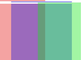
Layering translucent colors in p5.js and Processing is a fundamental way to create new, blended hues.
I'll use the method of layering semi-transparent colors to make complex gradients.
Now, the blendMode() function gives various effect on the mixed colors.
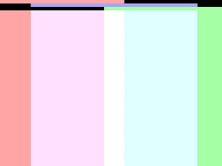
The blendMode(SCREEN) makes it brighter as you layer the colors. It behaves like light.
The blendMode(SUBTRACT) makes it darker as you layer the colors. It behaves like paints
blendMode(BLEND) (default blend-mode) is ideal for layering the semi-transparent colors. And I like the difference of mixed colors in the order of layering.
Seeking the Perfect Transition: From Linear to Organic
I'll explore how to create smoother color transitions by meticulously controlling transparency.
Level 1: Linear Gradients (The Basics)
It's the example that changes transparency in linear.
Linear transitions often feel a bit jarring, especially where the colors meet in the center.
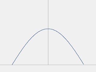
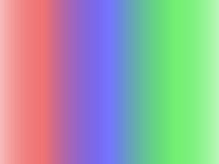
Level 2: Sine Curves (Smoother, but...)
It's the example that changes transparency in the sine curve.
The sine curve offers a smoother transition than the linear approach, though the edges can still feel somewhat abrupt.
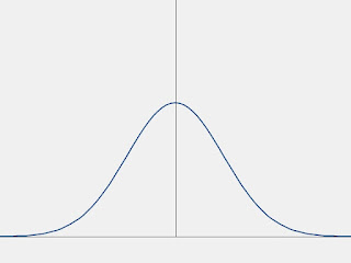
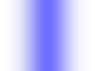
Level 3: Normal Distribution (The Gaussian Approach)
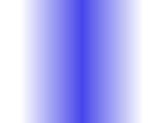
Could using a normal distribution make color transitions look more natural? Let's test this by applying a bell curve to our transparency values.
By using a normal distribution (Gaussian curve), we can achieve a much more natural, organic fade. A significant advantage of this method is the ability to fine-tune the gradient using mean and variance.
Applying Gaussian Gradients to Art
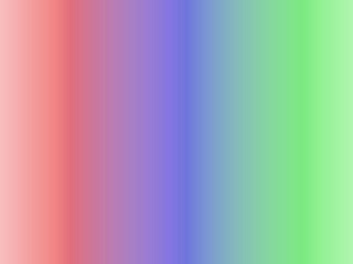
It's an example of artwork changing colors in the bell curve.
The colors are semi-transparent so the background can be seen through. You can make a composition by the background painting.
I placed the different color rectangles to be vertically arranged this time.
The p5.js Example Code
/**
 * Gradation of Blue.
 *
 * @author @deconbatch
 * @version 0.1
 * @license CC0
 * p5.js 1.5.0
 * created 2022.12.02
 */

function setup() {
  createCanvas(640, 1000);
  colorMode(HSB, 360, 100, 100, 100);
  noSmooth();
  noLoop();
  blendMode(BLEND);

  const yL = 0.7;

  // background
  fill(220, 90, 30, 100);
  rect(0, 0, width, height * yL);
  fill(220, 60, 90, 100);
  rect(0, height * yL, width, height);
  stroke(0, 0, 100, 100);
  line(0, height * yL, width, height * yL);

  // gradation
  gradateY(200, yL, 0.02, 80, createVector(55, 10, 100));
  gradateY(200, 0.1, 0.03, 80, createVector(260, 90, 5));
}

/**
 * gradateY : draw alpha gradation with the probability distribution function on Y-axis.
 * _divNum  : divide number.
 * _mean    : mean value of the probability distribution.
 * _vari    : variance value of the probability distribution.
 * _alpBase : alpha value on the top of the probability distribution curve.
 * _color   : x = hue, y = saturation, z = brightness
 */
function gradateY(_divNum, _mean, _vari, _alpBase, _color) {
  const divW = height / _divNum;
  const topV = 1 / sqrt(TWO_PI * _vari);
  noStroke();
  for (let i = 0; i < _divNum; i++) {
    let divRate = map(i, 0, _divNum, 0, 1);
    let density = exp(-pow(divRate - _mean, 2) / (2 * _vari)) / sqrt(TWO_PI * _vari);
    fill(_color.x, _color.y, _color.z, _alpBase * density / topV);
    rect(0, i * divW, width, divW);
  }
}
I utilized PVector to keep the gradateY() function's parameter list clean and manageable.
The Processing Example Code
/**
 * Gradation of Blue.
 *
 * @author @deconbatch
 * @version 0.1
 * @license CC0
 * Processing 3.5.3
 * created 2022.12.02
 */

public void setup() {
  size(640, 1000);
  colorMode(HSB, 360.0, 100.0, 100.0, 100.0);
  noSmooth();
  noLoop();
  blendMode(BLEND);

  float yL = 0.7;

  // background
  fill(220.0, 90.0, 30.0, 100.0);
  rect(0.0, 0.0, width, height * yL);
  fill(220.0, 60.0, 90.0, 100.0);
  rect(0.0, height * yL, width, height);
  stroke(0, 0, 100, 100);
  line(0, height * yL, width, height * yL);

  // gradation
  gradateY(200, yL, 0.02, 80.0, new PVector(55.0, 10.0, 100.0));
  gradateY(200, 0.1, 0.03, 80.0, new PVector(260.0, 90.0, 5.0));
}

/**
 * gradateY : draw alpha gradation with the probability distribution function on Y-axis.
 * _divNum  : divide number.
 * _mean    : mean value of the probability distribution.
 * _vari    : variance value of the probability distribution.
 * _alpBase : alpha value on the top of the probability distribution curve.
 * _color   : x = hue, y = saturation, z = brightness
 */
public void gradateY(int _divNum, float _mean, float _vari, float _alpBase, PVector _color) {
  float divW = height * 1.0 / _divNum;
  float topV = 1.0 / sqrt(TWO_PI * _vari);
  noStroke();
  for (int i = 0; i < _divNum; i++) {
    float divRate = map(i, 0, _divNum, 0.0, 1.0);
    float density = exp(-pow(divRate - _mean, 2) / (2.0 * _vari)) / sqrt(TWO_PI * _vari);
    fill(_color.x, _color.y, _color.z, _alpBase * density / topV);
    rect(0.0, i * divW, width, divW);
  }
}
Final Notes
The title drawing is my impression of the dawn I saw on my morning walk.
While this example focuses on the Y-axis, you can easily adapt the logic to the X-axis, specific areas, or even rotations. I hope you enjoy experimenting with these techniques!


